Flow Matching Policy Optimization with Mirror Descent and Entropy Constraints
Diffusion policies can represent rich, multimodal behaviour, but they are hard to train with online reinforcement learning. You cannot measure how random they are, so exploration relies on guesswork, and every update has to push gradients back through a long chain of denoising steps. We show that switching to flow matching removes both problems at once.
Our method, FMER, trains the policy with a simple weighted regression loss instead of backpropagating through the sampler, and it controls exploration with an exact entropy. On the FrankaKitchen benchmark, FMER completes nearly twice as many tasks as the strongest baseline on the hardest settings.
Why expressive policies, and why they are hard to train online
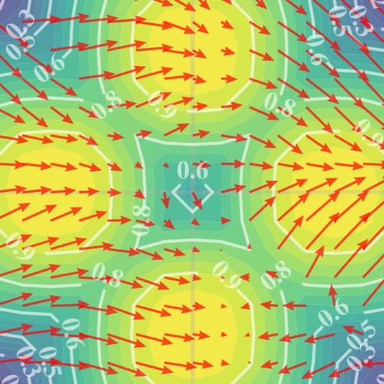
In continuous control, the standard Gaussian policy has a single peak. Many tasks, however, have several equally good ways to act in the same state: open the cabinet first or turn on the burner first; go left around the obstacle or go right. A single-peaked policy facing such a choice either commits to one option arbitrarily or averages between them and ends up doing neither well.
SAC Gaussian
DPMD Diffusion
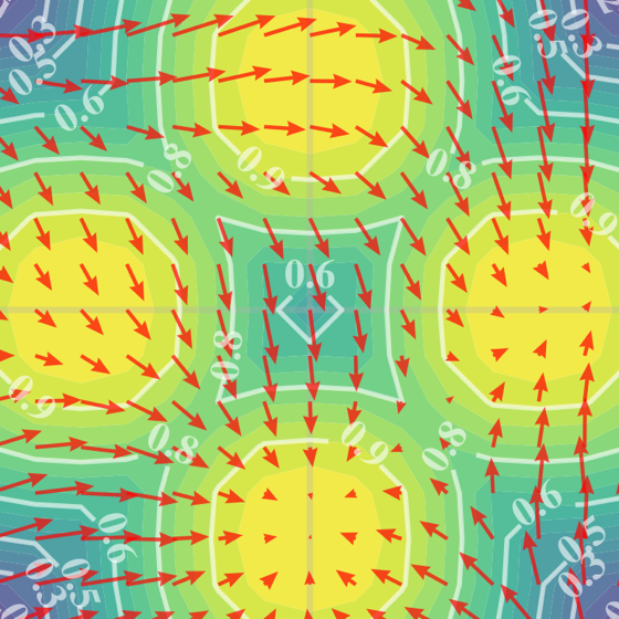
FMER Flow matching
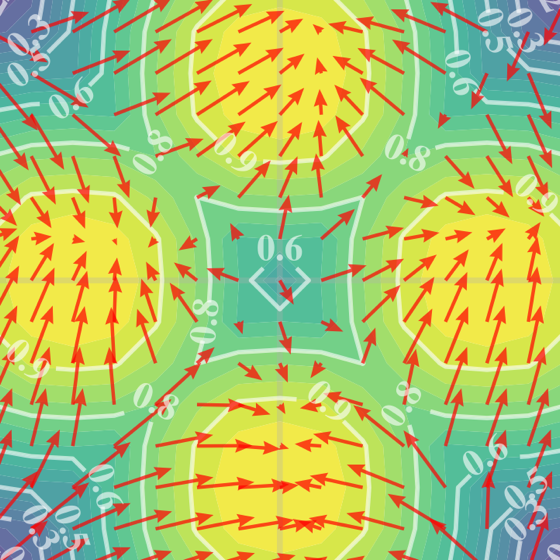
Generative policies fix this by turning random noise into actions, conditioned on the state. Diffusion policies first became popular for learning from fixed datasets. Using them in online RL, where the policy has to improve itself from rewards, runs into two problems:
- You can’t measure their randomness. Methods like SAC explore by keeping the policy’s entropy, its randomness, high. A diffusion model doesn’t tell you its entropy, so existing methods fall back on rough approximations that bias exploration.
- Training is slow and unstable. Improving the policy usually means backpropagating through every denoising step, which is expensive and noisy.
Flow matching generates actions by following a smooth, deterministic path from noise to action. A learned velocity field \(v_\theta\) moves a noise sample \(x_0\) step by step until it becomes an action:
\[\frac{d}{dt}x_t = v_\theta(x_t, t, s), \qquad x_0 \sim \mathcal{N}(0, I).\]Because this path is deterministic, the probability of each action can be computed. Existing flow-based RL methods still backpropagate through that path, though, and approximate the entropy to keep the cost down. FMER avoids both: training never simulates the path, and the entropy is exact.
Entropy-constrained policy mirror descent
FMER asks two things of each policy update. It should improve the policy, but not too much at once, and it should keep the policy random enough to keep exploring. Each request becomes one term of the objective.
Policy mirror descent (PMD) handles the first. The next policy \(\pi_{k+1}\) should pick actions with high advantage \(A\) (how much better an action is than the policy’s average), while staying close to the current policy \(\pi_k\):
\[\pi_{k+1} = \arg\max_{\pi}\; \mathbb{E}_{s\sim\mathcal{D}}\Big[\,\mathbb{E}_{a\sim\pi(\cdot \mid s)}\big[A^{\pi_k}(s,a)\big] \;-\; \tau\, D_{\text{KL}}\big(\pi(\cdot \mid s)\,\big\|\,\pi_k(\cdot \mid s)\big)\Big].\]The KL term is a trust region. The temperature \(\tau\) sets how far one update may move: a small \(\tau\) allows big steps, a large one keeps the policy near where it was. This problem has a closed-form solution, so the update can be written as a weighted maximum-likelihood problem: raise the log-probability of actions from the current policy, each weighted by \(\exp(A/\tau)\) and normalized per state by \(Z(s) = \mathbb{E}_{a\sim\pi_k}\big[\exp(A(s,a)/\tau)\big]\).
An entropy constraint handles the second. The entropy \(H(\pi)\) measures how random the policy is. We require it to stay above a target \(\bar{H}\), so that exploration doesn’t die out early:
\[\min_{\theta}\; -\mathbb{E}_{s,\,a\sim\pi_k}\Big[\frac{1}{Z(s)}\exp\!\big(A(s,a)/\tau\big)\,\log \pi_\theta(a \mid s)\Big] \quad \text{s.t.} \quad \mathbb{E}_{s}\big[H(\pi_\theta(\cdot \mid s))\big] \ge \bar{H}.\]Putting them together. As in SAC, the constraint becomes a penalty with a Lagrange multiplier \(\alpha\), which is tuned automatically: it grows when the entropy drops below the target and shrinks otherwise. Unlike SAC, the critic still estimates the plain discounted return, with no entropy bonus; entropy enters only through this constraint on the policy. So FMER is entropy-constrained policy optimization rather than full maximum-entropy RL. The result is one loss with one term per request:
\[\mathcal{L}_{\text{FMER}}(\theta) = \underbrace{\mathcal{L}_{\text{W-CFM}}(\theta)}_{\text{mirror descent}} \;+\; \alpha\, \underbrace{\mathcal{L}_{\text{ent}}(\theta)}_{\text{entropy}}.\]For a flow policy, neither term is easy as written. Both \(\log \pi_\theta\) and \(H(\pi_\theta)\) normally require running the generation path and differentiating through it. The next two sections replace each term with a loss that avoids this.
Ingredient 1: the mirror descent term as weighted flow matching
The closed-form solution of the mirror descent step is the target the policy should move towards:
\[\pi^*(a \mid s) \;=\; \frac{\pi_k(a \mid s)\, \exp\!\big(A(s,a)/\tau\big)}{Z(s)}.\]In words: take the current policy and boost the actions that are better than average. \(Z(s)\) just normalizes the result.
Fitting a flow policy to this target by maximum likelihood would mean differentiating through the whole generation path. Our theoretical result (Theorem 1) shows that this isn’t necessary. Sample some actions from the current policy, give each one the weight \(w(s,a) = \exp(A(s,a)/\tau)/Z(s)\), and train with the ordinary flow matching loss, weighted by those numbers:
\[\mathcal{L}_{\text{W-CFM}}(\theta) = \mathbb{E}\Big[\, w(s,a)\, \big\| v_\theta(x_t, t, s) - (x_1 - x_0) \big\|^2 \Big], \qquad x_1 = \operatorname{arctanh}(a),\; x_t = (1-t)x_0 + t x_1 .\]The velocity field is asked to point along the straight line from the noise \(x_0\) to the action \(x_1\), and high-weight actions count more. The best fit of this weighted loss is exactly the mirror descent target \(\pi^*\). Because the loss is a plain regression, there is no path to simulate and nothing to backpropagate through.
Weigh every candidate, not just the best one. In practice, FMER samples several candidate actions per state and lets the critic score them. Learning from all of them, in proportion to their weights, works better than copying only the top-scoring one: the top candidate may sit on a local peak, or the critic may simply overrate it.
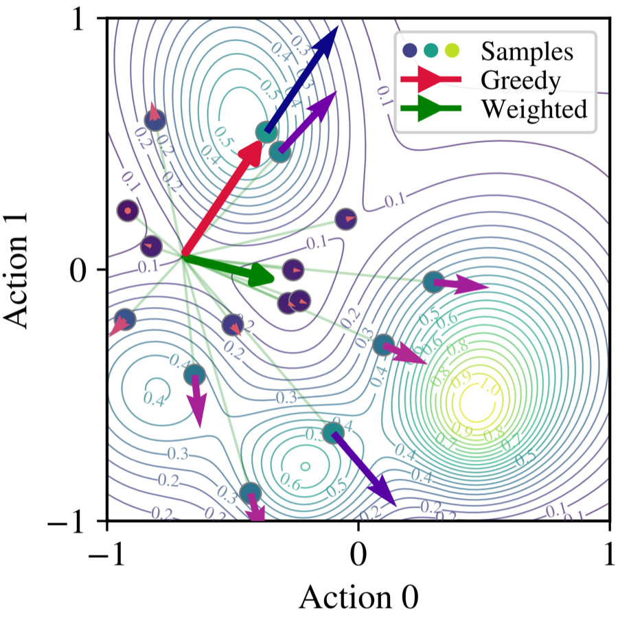
How to read it
- Contours are the true Q-values for one state. The best actions are the bright peak at the bottom right; the hill at the top left is only a local peak.
- Dots are 16 candidate actions sampled from the policy. The small arrows show how much weight each one gets.
- Greedy copies the single best sample and climbs the local peak.
- Weighted (FMER) pools all the candidates and heads towards the global optimum.
Step size, tuned automatically. If \(\tau\) is too large, the policy barely moves; if it is too small, a single candidate takes over. FMER measures how evenly the weights are spread with the effective sample size, \(\text{ESS} = 1/\sum_l \hat{w}_l^2\), which runs from 1 (one candidate dominates) to \(M\) (all \(M\) candidates count equally). It adjusts \(\tau\) to keep ESS at a target value, so it needs no per-environment tuning.
Ingredient 2: the entropy term, computed exactly
Because the flow is deterministic, its entropy can be computed exactly by tracking how the flow stretches or squeezes space as it carries noise to actions. That stretching is the divergence of the velocity field, integrated along the path:
\[H(p_1) = H(p_0) + \int_0^1 \mathbb{E}_{x_t}\big[\nabla_x \cdot v_\theta(x_t, t, s)\big]\, dt .\]There is a catch that is easy to miss. Robots need bounded actions, so FMER squashes its output into the valid range with \(a = \tanh(x_1)\). That squashing distorts the probabilities, and what we care about is the randomness of the actual action, not of the value before squashing. Proposition 1 gives the corrected divergence in action space:
\[\nabla_a \cdot v^a = \nabla_x \cdot v_\theta \;-\; 2\,\big\langle \tanh(x),\, v_\theta(x, t, s) \big\rangle .\]The second term pushes back when the policy piles probability onto the action limits. Maximizing entropy means minimizing its negative, so the entropy loss is the corrected divergence with a minus sign:
\[\mathcal{L}_{\text{ent}}(\theta) = -\,\mathbb{E}_{t,\,x_t}\Big[\nabla_x \cdot v_\theta(x_t, t, s) \;-\; 2\,\big\langle \tanh(x_t),\, v_\theta(x_t, t, s) \big\rangle\Big].\]Like the mirror descent loss, it is evaluated along the same straight paths, so the flow never has to be simulated. Plugging both losses into the combined objective \(\mathcal{L}_{\text{FMER}}\) gives the full training signal.
The training loop
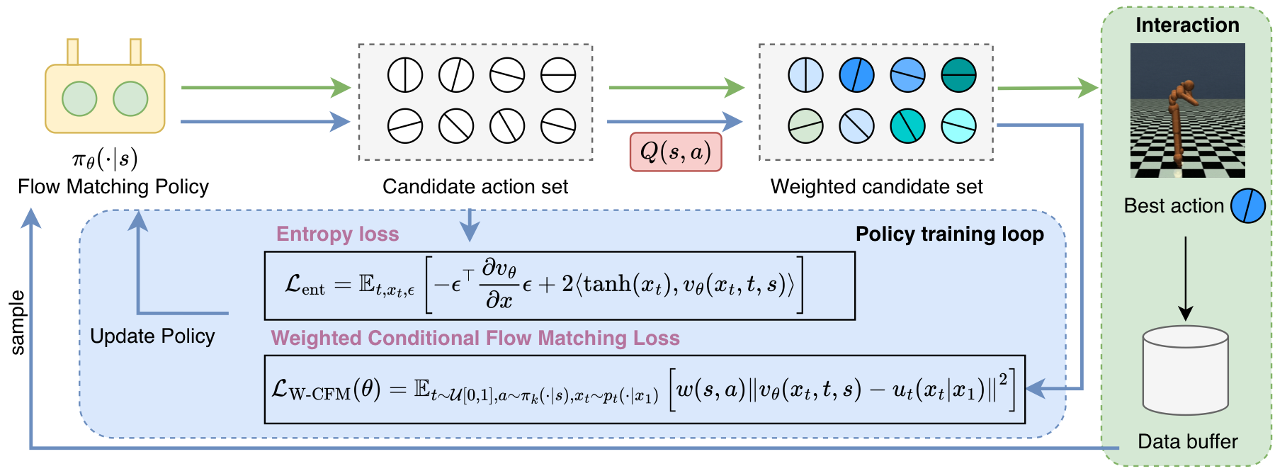
Each training step does four things:
- Act. Generate a handful of candidate actions, execute the one the critic likes best, and store the result.
- Critic. Update the estimates of how good each action is.
- Policy. Weight the candidates by the critic’s scores and update the policy with the weighted flow matching loss plus the entropy term.
- Tune. Adjust \(\alpha\) to track the target entropy and \(\tau\) to track the target ESS.
Results
We compared FMER with eight baselines that use Gaussian, diffusion or flow policies. Every method was trained for one million steps, over 5 random seeds.
FrankaKitchen (sparse reward). A robot arm in a simulated kitchen has 280 steps and earns a reward only when it finishes a sub-task, such as moving the kettle. With rewards this rare, exploration is the main challenge. We test sets of 1, 2, 4 and 7 tasks. FMER is best on 1, 4 and 7 tasks and level with the best baseline on 2 (48% vs. 50%). The gap widens as tasks are added: with 7 tasks, FMER completes 40% vs. 23% for the next best method.
FrankaKitchen: normalized task completion (%)
Mean over 5 seeds. FMER keeps its completion rate as the task set grows; the baselines fall away.
Show all methods as a table
| Method | N = 1 | N = 2 | N = 4 | N = 7 |
|---|---|---|---|---|
| PPO | 2.0 | 0.0 | 1.0 | 8.6 |
| SAC | 40.0 | 32.0 | 2.5 | 12.3 |
| TD3 | 0.0 | 11.0 | 15.0 | 5.7 |
| DIPO | 0.0 | 33.0 | 14.5 | 23.1 |
| DPMD | 60.0 | 50.0 | 25.0 | 20.6 |
| QVPO | 0.0 | 0.0 | 0.0 | 18.9 |
| SAC-Flow | 0.0 | 0.0 | 0.0 | 0.6 |
| FLAME | 8.0 | 10.0 | 6.5 | 18.3 |
| FPO | 0.0 | 1.0 | 0.0 | 0.0 |
| FMER | 80.0 | 48.0 | 46.5 | 40.3 |
The baselines fail in telling ways. SAC falls apart once there are several task orders to choose from. DPMD locks onto its early successes and can’t move on. And the methods with approximate entropy (QVPO, SAC-Flow) explore poorly exactly where exploration matters most.
MuJoCo (dense reward). These standard locomotion tasks check that FMER’s extra machinery doesn’t hurt on easier problems. FMER scores highest on HalfCheetah and Walker2d and second on Humanoid. It falls behind on Hopper, a simple task where its extra exploration goes on longer than needed.
MuJoCo-v5: episode return
Mean over 5 seeds, sorted within each environment. Scales differ per environment, so compare ranks, not bar lengths across panels.
Show as a table
| Method | Hopper | HalfCheetah | Walker2d | Humanoid |
|---|---|---|---|---|
| PPO | 1198 ± 361 | 5983 ± 811 | 4598 ± 222 | 812 ± 78 |
| SAC | 3319 ± 133 | 10295 ± 1170 | 4442 ± 537 | 5327 ± 59 |
| TD3 | 3662 ± 62 | 9497 ± 901 | 4888 ± 631 | 318 ± 208 |
| DIPO | 3409 ± 297 | 9516 ± 1417 | 5029 ± 217 | 5087 ± 100 |
| DPMD | 3398 ± 278 | 10706 ± 818 | 4901 ± 352 | 5085 ± 28 |
| QVPO | 3423 ± 413 | 10310 ± 1398 | 4846 ± 398 | 5064 ± 49 |
| SAC-Flow | 2931 ± 510 | 9933 ± 255 | 5234 ± 729 | 4857 ± 2763 |
| FLAME | 2594 ± 432 | 10901 ± 1478 | 4407 ± 144 | 5207 ± 346 |
| FMER | 2913 ± 643 | 12332 ± 904 | 5283 ± 438 | 5286 ± 65 |
What matters. Removing FMER’s parts one at a time shows that each one earns its place:
- Entropy constraint. Without it, the policy turns almost deterministic early in training and completes 0% of the 7-task kitchen.
- Weights. With equal weights, the policy just imitates its own samples, and performance drops.
- \(\tanh\) squashing correction. Replacing \(\tanh\) with hard clipping, and so dropping the correction, lowers every MuJoCo score, HalfCheetah from 12.3k to 7.7k.
FMER also trains faster than the diffusion baselines, though slower than the lightest flow-based method.
Limitations
- Speed. FMER trains faster than the diffusion baselines but slower than SAC-Flow, because it integrates more ODE steps (10 vs. 4) and computes the exact entropy instead of a cheaper surrogate.
- Simulation only. All experiments are in simulation. Whether the gains carry over to real robots is still an open question.
Takeaway
Choosing between diffusion and flow matching is not just about how fast you can sample. For online RL, flow matching’s deterministic path is what makes a principled algorithm possible: the policy update becomes a weighted regression, and the policy’s randomness becomes something you can measure and control. FMER puts both pieces together, and the gains show up exactly where exploration is hardest.
Citation
@inproceedings{gao2026fmer,
  title     = {Flow Matching Policy Optimization with Mirror Descent and Entropy Constraints},
  author    = {Gao, Ting and Orfanoudakis, Stavros and Lin, Nan and Daamen, Winnie and Hoogendoorn, Serge and Isufi, Elvin},
  booktitle = {Advances in Neural Information Processing Systems},
  year      = {2026}
}